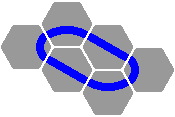
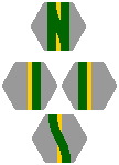
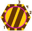
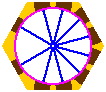
§11. Single-segment pieces. In this system, all curves are circular and of the same radius, but of a 60° angle rather than 45°. If the radius, R, is 200mm then such a curve fits into a regular hexagon of edge 133.33mm [= 2 × R ÷ 3], where the center line of the track meets the midpoints of two edges, and the tangent to the curve is perpendicular to the edge. With this radius, the length of a curved piece along its center line is 200 × pi ÷ 3 millimeters, approximately 209.44. The drawings continue to assume a track width of 40mm.

This hexagon with its component track can be turned any of six directions:

Figure 11-1

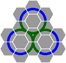
The virtue of this plan is that the regular hexagon is tessallable in the plane. To assemble layouts becomes easy:

Figure 11-2	Figure 11-3

The straight piece will inevitably be of length 2 × R ÷ √3. When R is 1 quintimeter, this works out to 230.94mm.

Figure 11-4

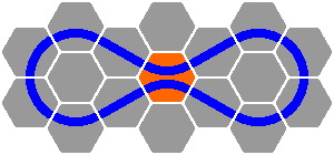
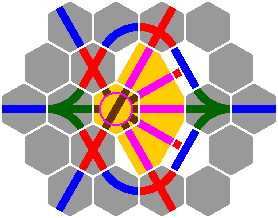
Note that the hexagon is not physically manufactured — it is simply a concept for demonstrating how track segments will fit. Hence the center area in the next figure [highlighted in orange] is two separate pieces of track, and not one large hexagonal assembly. Neither is it a gantlet, unless the track is wider than 62mm [= 800 ÷ √3 − 400].

Figure 11-5

Overpasses are possible; compare figure 11-6a to figure 2-4. Figure 11-6b is like figure 11-6a except that display of the hexagons has been suppressed — this simplification will be often be performed. Note also that the hexagonal structure has been turned 90° to fit better on the screen.

Figure 11-6a	Figure 11-6b

It is possible to create a curve of small radius [R ÷ 3] as in figures 11-7 and 11-8; if R is 200mm, then R ÷ 3 is 66.67mm. This curve will align properly with the curved and straight pieces already introduced [figure 11-9]. Because train cars of 100mm length will likely have difficulty negotiating such a sharp curve, it will not be investigated further in this report.

Figure 11-7	Figure 11-8	Figure 11-9

Note that the 60° system does not entail anything like the primary or secondary series of the 45° system; it is qualitatively different. Much as √2 is found throughout the 45° system, √3 is fundamental to the 60° system. In a 36° system, √5 would be the corresponding number.

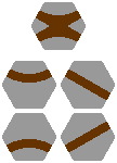
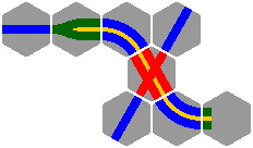
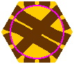
§12. Crossings. There are five crossing pieces, shown in figure 12-1.

Figure 12-1

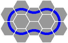
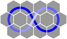
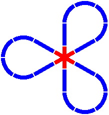
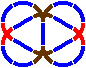
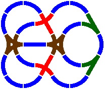
Figure 12-2 is a classical pattern, while figure 12-3 substitutes an overpass for one of the crossing segments. Figure 12-4 is a well-known design, consisting of three disjoint circles.

Figure 12-2	Figure 12-3	Figure 12-4

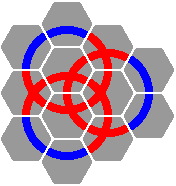
Figure 12-5 demonstrates that considerable complexity is possible. In the 60° scheme, verifying that the pieces do actually meet does not require detailed calculations, as it would in the 45° system. Instead, one need merely fit the hexagons together.

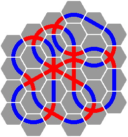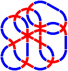
Figure 12-5a	Figure 12-5b

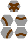
§13. Switches. In the 60° system, there are precisely seven switches, in contrast to the 45° system where the number is unbounded.

Figure 13-1

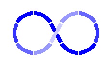
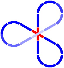
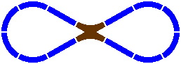
Figure 13-2 depicts an oval-eight, while figures 13-3 and 13-4 are variations on 12-4 that render the three circles conjoint.

Figure 13-2	Figure 13-3	Figure 13-4

§14. Miscellaneous pieces.

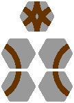
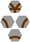
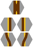
14A. Several combinations of switch and crossing are feasible. The piece at the top of figure 14-1 is a combination of the four segments below it; the layout in figure 14-2 shows one way to use this crossing switch. Figures 14-3 through 14-8 are similarly organized.

Figure 14-1	Figure 14-2

Figure 14-3	Figure 14-4

Figure 14-5	Figure 14-6

Figure 14-7	Figure 14-8

What might be considered the ultimate piece has nine segments, and can be viewed as the union of the six segments of figure 11-1 with the three of 11-4. Unclear, however, is whether such a complicated piece would actually work. If track is implemented as grooves cut into a base, there may be so many grooves that train wheels receive insufficient guidance and wander off course. If instead track is more realistically constructed as rails, there may be so may cuts in the rails [for allowing crossing wheel flanges to pass] that trains derail. This piece is not illustrated on this page because it is too complicated to effectively render in the available resolution, but it is included in a gallery of pieces possible under this system.

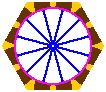
14B. Design of the turntable is obvious; the exact diameter of the disk can be selected according to practical considerations. Figure 14-9 shows disks with various arrangements of segments. In figures 14-9d and 14-9e, the radius of the curve is necessarily less than 1 quintimeter, because of the width of the ring.

	Figure 14-9b	Figure 14-9d
Figure 14-9a	Figure 14-9c	Figure 14-9e

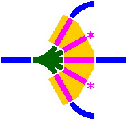
14C. A basic roundhouse is shown in figure 14-10; the asterisks denote segments that do not fit into the 60° system. Figure 14-11 includes a tessellation to show how the roundhouse fits; note that there is room for barricades on its convex side.

Figure 14-10	Figure 14-11

§15. Double tracking.

15A. The 60° system can be extended to allow two parallel tracks within a hexagon. A fundamental use is to model a siding:

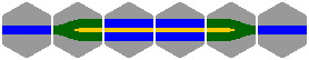
Figure 15-1

The yellow filling between segments means that they are physically connected, and count as one piece. Nothing prevents double tracks from being curved, having crossings, or ending in ramps:

Figure 15-2

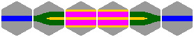
Figure 15-3 shows segments enclosed in a carbarn. As in figure 8-8, the color pink signifies a section of track inside a building.

Figure 15-3

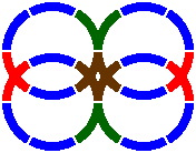
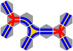
When double-tracked pieces meet, various configurations are possible. In some cases, there is ambiguity about whether coloring in a double-tracking diagram should be blue [for a plain segment] red [crossing], green [switch], brown [crossing plus switch], or some combination of colors.

Figure 15-4	Figure 15-5

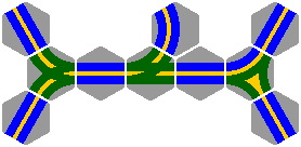
Single and double crossovers can be used. Shown are decompositions in the manner of figure 14-1.

Figure 15-6a	Figure 15-6b

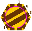
15B. Figure 15-7 is an obvious design for the double-track turntable. A train car entering at outer portal 1 can leave at outer portal 2 [figure 15-7b] without pivoting, or at outer portal 3 [figure 15-7c] after pivoting. Unfortunately, it cannot leave at outer portal 4 [figure 15-7d] without negotiating a sharp corner at inner portal 4, which will probably cause the car to become stuck.

Figure 15-7a	Figure 15-7b scale 2x	Figure 15-7c scale 2x	Figure 15-7d scale 2x

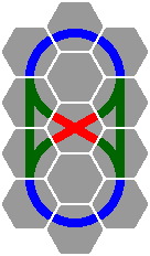
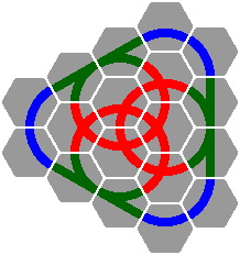
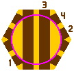
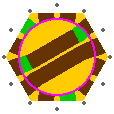
One way to eliminate this corner is to ensure that every track, when it comes to inner portal, is perpendicular to the disk-ring boundary. Such is illustrated in figure 15-8, where the hexagons [as always] have an edge of 133.33mm.

• The inner radius [pink circle] of the turntable is 94.28mm [= 400 ÷ (3 × √2)].
• All twelve track segments on the ring are circular arcs of radius 94.28mm and angle exactly 15°. Each arc is centered on a corner of the hexagon.
• Within the disk, each segment has a straight portion of 133.33mm connecting two arcs congruent to those on the ring. Whenever the disk is in one of its twelve functional positions, the center of each of these arcs lies on one of the gray dots of figure 15-8b. These dots are the corners of a regular dodecagon, and six of them are also the corners of the hexagonal turntable.

Four instances of this subtle curve are highlighted in green in figure 15-8b. Figure 15-8c reveals that the inner portals lie at uniform 30° intervals. This feature somewhat increases the chance, after one train car has left the turntable, that the disk will be correctly oriented for the next car. The 30° spacing also allows the two disk segments to be assigned to different sets of double tracks, as in figure 15-8d. [The turntable of figure 14-11 also has 30° spacing in part, but the segments are aligned on the turntable differently.]

Figure 15-8a	Figure 15-8b scale 2x	Figure 15-8c scale 2x	Figure 15-8d

These specifications mean that, on ordinary double track as in figure 15-1, the center-to-center distance between the parallel tracks will have to be 55.23mm [= (400 × √2 − 400) ÷ 3]. If track is 40mm wide, the median becomes 15.23mm [= 55.23 − 40]. With these numbers, the radii [to center line] of the curved segments in figure 15-2 are 172.39mm [= 200 − 55.23 ÷ 2] and 227.61mm [= 200 + 55.23 ÷ 2]. The median within the disk of figure 15-8 turns out to be only 2.38mm [= 15.23 − 4 × 94.28 × (1 − cos15°)]. Naturally, the turntable could be implemented with other radii or center points for the curves, generating a different median size.

A crossing track is feasible [figure 15-9]; in this example the added segment is entirely straight.

Figure 15-9a	Figure 15-9b scale 2x

If single-track approaches are mixed with doubles [figure 15-10a] the consistent 30° spacing of inner portals [figure 15-8c] will be lost [figure 15-10b]: some angles will be 45° or 60°. To restore uniformity, switches can be used [figure 15-10c] to convert single-track approaches to double.

Figure 15-10a	Figure 15-10b scale 2x	Figure 15-10c

The reader may have concluded that the design of a proper double-track turntable is rather complicated. However, children should find this piece of equipment very easy to use, and even advanced hobbyists will rarely need to examine the mathematical subtleties involved.